MS Excel Lesson 2

Sorting and filtering data in Excel are fundamental tasks that allow you to organize and analyze your data more efficiently. Here's a brief explanation of both:

YOU CAN SAVE THE LESSON FILE BY CLICKING ON THE DOWNLOAD BUTTON AT THE END OF THE LESSON

Sorting Data in Excel

Sorting data means arranging it in a specific order, typically alphabetically, numerically, or by date. You can sort data in ascending or descending order. Here’s how to do it:

1. Select the Data: Click on a cell within the column you want to sort. If you want to sort multiple columns, select the entire range of data to sort.
2. Sort Using the Ribbon:
   • Go to the "Data" tab on the ribbon.
   • Use the "Sort A to Z" (ascending order) or "Sort Z to A" (descending order) buttons for simple sorting based on one column. This will sort your selected data or the entire dataset if only one cell is selected.
   • For more complex sorting (e.g., sorting by multiple columns), click the "Sort" button to open the Sort dialog box. Here, you can add levels and determine the specific order for each column you want to sort by.
3. Sort Using Right-Click:
   • Right-click within the cell range you want to sort.
   • Choose "Sort" from the context menu and then select your sorting preference.

Filtering Data in Excel

Filtering data allows you to display only the rows that meet certain criteria, hiding the others. This is useful for analyzing parts of your dataset without deleting or moving data around. Here’s how to apply filters:

1. Select the Data: Click on any cell within your dataset. If your data has headers, it’s best to click one of them.
2. Apply Filter:
   • Go to the "Data" tab on the ribbon.
   • Click the "Filter" button. This adds dropdown arrows to each of your column headers (or the first row of your data if headers are not defined).
3. Use the Filter Dropdown:
   • • Click on the dropdown arrow next to the column header you want to filter by.
     • You will see a variety of filtering options, including checkboxes for each unique item in the column. Uncheck the box next to "(Select All)" to deselect all items, then check the boxes next to the values you want to display.
     • You can also use text filters or number filters to set more specific criteria, such as containing specific text or being greater than a certain number.
    

Tips for Sorting and Filtering

• Headers: When sorting or filtering, make sure your data has headers, and Excel recognizes them as such. This makes your actions clearer and prevents accidental sorting of the header row as data.
• Data Integrity: Especially when sorting, ensure your data is contiguous (no blank rows or columns) to prevent accidental partial sorting, which can scramble your data.
• Sorting and filtering are non-destructive: Filtering hides rows without deleting them, and sorting can be undone with the Undo command (Ctrl + Z).

By mastering sorting and filtering, you'll be well-equipped to handle a wide range of data analysis tasks in Excel.  

Chapter 2: Data Validation

Data Validation in Excel is a feature that allows you to control the type of data or the values that users can enter into a cell. These controls can include a wide range of criteria, such as restricting entries to specific numbers, dates, or lists, and even custom validations based on formulas. Data Validation is crucial for maintaining data integrity, ensuring consistency, and reducing errors in data entry processes.

How Data Validation is Useful:

• Maintain Data Integrity: By restricting the type of data that can be entered into cells, you ensure that your datasets are accurate and consistent. For example, preventing accidental entries of text in a numeric field.
• Simplify Data Entry: Using drop-down lists limits choices to certain items, making it easier for users to fill out forms or datasets without needing to know all possible valid entries.
• Prevent Data Entry Errors: By setting specific numerical ranges or date boundaries, you can prevent out-of-range entries. This is especially useful in scenarios like scheduling, budgeting, and inventory management.
• Customize Input Requirements: With custom formulas, you can create complex validation criteria, such as preventing duplicate entries in a column or ensuring that a value in one cell is greater than the value in another.
• Provide Input Guidance: You can set up input messages that appear when a cell is selected, guiding users on what type of data is expected. This can include instructions, data formats, or examples.
• Feedback on Invalid Data: When users enter data that violates a validation rule, you can display an error alert that explains what was wrong with the input and how to correct it.

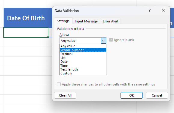
How to Set Up Data Validation:

1. Select the Cells: Start by selecting the cells or range where you want to apply data validation.
2. Open Data Validation Dialog Box: Go to the Data tab on the Ribbon, and click on Data Validation in the 'Data Tools' group.
3. Specify Validation Criteria:
   • In the Settings tab, choose the type of validation (e.g., whole number, decimal, list, date, time, text length, or custom).
   • Specify the criteria (e.g., between, less than, greater than for numbers, or a source range for lists).
4. Input Message (optional):
   • Switch to the Input Message tab to create a message that appears when the cell is selected, guiding users on the expected input.
5. Error Alert (optional):
   • In the Error Alert tab, you can customize the message that appears when someone tries to enter invalid data. You can choose the style of the alert (Stop, Warning, or Information) and provide a title and error message.
6. Finalize: Click OK to apply the settings.

Examples of Use Cases:

• Employee Scheduling: Ensure that dates and shifts entered fall within an operational calendar and predefined shifts.
• Financial Budgeting: Restrict budget line items to certain numerical ranges or percentages.
• Inventory Management: Ensure product codes or quantities entered are within a valid range or match a predefined list.
• Surveys and Forms: Use drop-down lists for consistent responses and custom validations to ensure that certain criteria are met (e.g., age ranges, zip codes).

By leveraging Data Validation, Excel users can significantly reduce the time and effort required to clean and analyze data, leading to more reliable and meaningful insights.

Chapter 3: Text to Column

"Text to Column" in Excel is a feature that allows you to split the contents of one column into multiple columns based on a specific delimiter or a fixed width. This tool is incredibly useful for reformatting and organizing data that comes in a single column into a more usable and structured format. Here's how it can be useful:

1. Splitting Combined Data

Often, data imported from other sources (like CSV files) or copied from other applications may contain multiple pieces of information within a single cell. For example, a cell might contain full names, where you might want to split first names and last names into separate columns. Text to Column can do this based on a space delimiter.

2. Data Cleaning

It aids in cleaning data. For instance, if you have a list of dates in a format not recognized by Excel, you can use Text to Column to split the date components and then recombine them in a format that Excel recognizes.

3. Formatting Consistency

When importing or copying data from different sources, it might not always adhere to the format you need for analysis or reporting. Text to Column can help reformat this data by splitting and then allowing you to recombine or rearrange the data as needed.

4. Extracting Specific Information

In scenarios where you have a column with structured text (like an email address), and you need to extract specific parts (like usernames before the @ symbol), Text to Column can be set to use the @ as a delimiter to separate the usernames into a new column.

5. Preparation for Analysis

Before performing data analysis, it’s often necessary to restructure data sets. Text to Column helps in breaking down complex, concatenated data into more analyzable chunks, like separating address fields into street, city, and zip code columns.

How to Use Text to Column in Excel:

1. Select the column of data you wish to split.
2. Go to the Data tab on the Ribbon.
3. Click on Text to Columns.
4. Choose Delimited if your data is separated by characters such as commas, tabs, or spaces. Choose Fixed Width if you want to split the data based on specific positions.
5. If you chose Delimited, select the delimiter(s) that apply. If you chose Fixed Width, set the column breaks.
6. Click Finish after configuring any additional options such as data formats for the new columns.

This feature, with its straightforward implementation, can significantly reduce manual data entry and manipulation, making it a go-to tool for preliminary data preparation and cleaning tasks.

Chapter 4: Go to Special

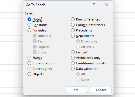
"Go To Special" in Excel is a powerful feature that allows you to quickly select specific types of cells within a worksheet based on certain criteria, without having to manually sift through your data. This feature can greatly enhance your productivity and efficiency when working with complex Excel sheets. Here's how "Go To Special" can be useful:

1. Selecting Cells with Formulas

You can use "Go To Special" to select all cells that contain formulas. This is particularly useful when you need to review or modify formulas across a large spreadsheet.

2. Highlighting Constants

If you need to identify all cells containing constants (values not derived from formulas), "Go To Special" can isolate these cells. This can be helpful for verifying or updating data entries.

3. Finding Blank Cells

"Go To Special" can select all blank cells within a specified range. This feature is incredibly useful for quickly identifying gaps in your data or preparing ranges of cells for new data entry.

4. Selecting Cells with Data Validation

For spreadsheets utilizing data validation rules, "Go To Special" can highlight cells that have data validation applied. This makes it easier to review or adjust these rules across your dataset.

5. Isolating Comments or Notes

If your spreadsheet contains comments or notes, you can use "Go To Special" to select these cells. This is handy for reviewing annotations or instructions left by yourself or others.

6. Selecting Formulas that Return an Error

This is particularly useful for troubleshooting and fixing errors in a large worksheet. "Go To Special" can quickly identify all cells where formulas result in errors.

7. Highlighting Visible Cells Only

In sheets with hidden rows or columns, "Go To Special" can select only those cells that are visible. This is crucial for applying changes or formatting only to the part of the sheet that is visible.

How to Use Go To Special in Excel:

1. Press Ctrl + G or F5 to open the "Go To" dialog box, then click "Special" or you can directly access it via the Home tab → Find & Select → Go To Special.
2. Choose the type of cells you want to select (formulas, constants, blanks, etc.).
3. Click OK. Excel will then select the cells that match your criteria.

"Go To Special" is a versatile tool that can streamline tasks like formatting, analyzing, or cleaning up your data. By efficiently targeting specific cell types, you can save time and avoid the manual labor of sifting through potentially thousands of cells. Whether you're an Excel novice or a seasoned pro, incorporating "Go To Special" into your workflow can significantly boost your productivity.

Chapter 5: Paste Special

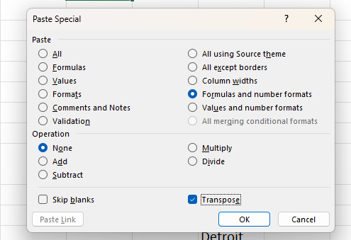
"Paste Special" in Excel is a feature that offers advanced options for pasting data from the clipboard into your worksheet. Unlike the standard paste operation, which simply duplicates the copied content, Paste Special allows you to selectively paste only certain elements of the copied data (such as its value, format, or formula) or to perform operations on the pasted data, such as adding it to or subtracting it from the existing values. This functionality can be extremely useful in a variety of situations:

1. Pasting Values Only

When you copy a cell with a formula and just want to paste the resulting value, not the formula itself, Paste Special comes in handy. This is particularly useful when preparing data for reporting or when you need to share data without the underlying calculations.

2. Pasting Formulas Only

Conversely, if you want to copy the formula from one cell to another without copying the formatting or the value, you can use Paste Special to paste only the formula. This is helpful when applying the same calculations across different datasets.

3. Pasting Formatting

If you've spent time formatting a cell or range of cells and want to apply the same formatting elsewhere, Paste Special allows you to copy and paste just the formatting. This includes fonts, colors, borders, and number formatting, ensuring consistency across your document without altering the content.

4. Transposing Data

Transposing data means switching rows to columns or vice versa. Paste Special offers an easy way to transpose data without manually re-entering it, saving time and reducing the risk of errors.

5. Performing Operations While Pasting

Paste Special can apply mathematical operations (Add, Subtract, Multiply, Divide) to the pasted data based on the values in the destination cells. For example, if you have a column of numbers and you want to increase them by a certain percentage, you can copy the percentage and use Paste Special to multiply the existing values by this percentage in one step.

6. Skip Blanks

This option allows you to paste data into a range while ignoring blank cells in the copied range. It's useful for filling in gaps without overwriting existing data.

7. Paste Link

This creates a reference to the copied data. Instead of pasting the actual data or formula, it inserts a link to the original cell. Any changes made to the original cell will automatically update in the cell where the link was pasted.

How to Use Paste Special in Excel:

1. Copy the cell or range of cells you want to work with.
2. Select the destination cell or range.
3. Right-click and choose Paste Special, or go to the Home tab, click the Paste dropdown, and select Paste Special.
4. Choose the option that suits your needs and click OK.

Incorporating Paste Special into your Excel workflow can significantly enhance your productivity, allowing for sophisticated data manipulation and formatting with just a few clicks. Whether you're consolidating data, reformatting spreadsheets, or performing complex calculations, Paste Special offers a flexible and powerful set of options to achieve your goals efficiently.

Chapter 6: Fill Series

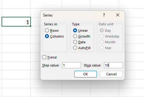
"Fill Series" in Excel is a feature that allows you to automatically fill cells with a series of data, such as numbers, dates, or custom sequences. It's particularly useful when you need to quickly generate a sequence of values without manually typing them one by one. Here's how it can be helpful:

1. Sequential Numbering

You can use Fill Series to quickly generate a sequence of numbers in ascending or descending order. For example, if you have a list starting from 1 and need to continue the sequence, you can use Fill Series to populate the next numbers automatically.

2. Auto-filling Dates

If you need to create a series of dates, such as days of the week, months, or years, Fill Series can automatically generate these dates based on the initial selection. This saves time and ensures accuracy when working with date-based data.

3. Custom Sequences

Fill Series allows you to create custom sequences of data. For instance, you can specify a pattern like repeating numbers or a specific pattern of text. This flexibility is handy for creating unique sequences tailored to your needs.

4. Incrementing Values

You can use Fill Series to increment values by a specific amount. This is useful for scenarios like generating a series of prices, quantities, or other numerical data with a consistent increment.

5. Copying Formats

Fill Series can not only fill cells with data but also copy formatting. For example, if you have a cell with a specific format (such as bold, italic, or colored), you can use Fill Series to copy this formatting to adjacent cells.

Benefits:

• Efficiency: Saves time compared to manually typing each value.
• Accuracy: Reduces the risk of errors when generating sequences of data.
• Customization: Allows for the creation of custom sequences tailored to specific requirements.

In summary, Fill Series is a handy feature in Excel for quickly generating sequential data, dates, or custom sequences with ease and accuracy, making it an essential tool for spreadsheet users working with large datasets.

Chapter 7: Flash Fill

"Flash Fill" is a feature that helps automatically fill data based on patterns it recognizes in adjacent columns. It's particularly useful for tasks where you need to extract or transform data based on a consistent pattern. Here's how it can be helpful:

1. Data Extraction

Flash Fill can automatically extract specific parts of data from one column and fill them into adjacent columns. For example, if you have a column with full names, Flash Fill can recognize patterns such as first name followed by last name and automatically extract them into separate columns.

2. Data Transformation

It can transform data from one format to another based on a pattern. For instance, if you have a column with dates in one format (e.g., "January 1, 2022") and need them in another format (e.g., "01/01/2022"), Flash Fill can recognize the pattern and transform the data accordingly.

3. Data Cleaning

Flash Fill can help clean and standardize data by recognizing patterns and applying consistent formatting. For example, if you have a column with phone numbers in various formats, Flash Fill can reformat them to a standard format.

4. Combining Data

It can concatenate data from multiple columns into a single column based on a pattern. For example, if you have separate columns for first name and last name, Flash Fill can combine them into a single column for full name.

5. Splitting Data

Conversely, Flash Fill can split data from one column into multiple columns based on a pattern. For example, if you have a column with addresses in one cell, Flash Fill can recognize patterns such as street address, city, state, and ZIP code and split them into separate columns.

How to Use Flash Fill in Excel:

1. Enter the desired pattern in the adjacent column(s) based on which you want Excel to recognize and autofill data.
2. Start typing the desired pattern in the first cell of the adjacent column(s).
3. Press Ctrl + E or go to the Data tab → Flash Fill and click on it.
4. Excel will automatically detect the pattern and fill the adjacent cells accordingly.
5. Review the filled cells for accuracy and make adjustments if necessary.

Benefits:

• Time-saving: Automates repetitive data entry and manipulation tasks.
• Accuracy: Reduces the risk of errors associated with manual data entry.
• Ease of Use: No complex formulas or coding required; can be used by non-technical users.

Flash Fill is a powerful tool for quickly and accurately manipulating data based on recognizable patterns, making it a valuable asset for anyone working with data in Excel.

SAVE THE LESSON FILE BY CLICKING ON THE DOWNLOAD BUTTON ⬆️